HSPEXP+ Released!

I was recently notified that the new version of HSPEXP, HSPEXP+, has been released by AQUA TERRA!  They retained a lot of the work I did coding up the old advice (and adding some new advice) and designing the user interface so listed me as an author.  I'm excited to see all of their efforts come to fruition, and for the modeling world to finally have a modern version of my favorite calibration system!  Go check it out!

ArcGIS 10.1 - Geoprocessing Quirks and Solutions

Well, this one stumped me for a good week, so I figured time to return to the blog!


At long last, my colleagues at the City all upgraded to ArcGIS 10.1 SP1.  So I figured it was high time I follow suit.


Unbeknownst to me at the time, the 10.1 upgrade apparently did some small tweaks to the geoprocessor's background processing.  As a result, certain tools no longer worked when run synchronously - most notably for me, the Dissolve and Erase tools.  I had to call ESRI support before we figured out this one - see my StackExchange post on the subject.  Long story short, this was a known bug (presumably fixed at 10.2, which we won't be upgrading to for a LOOOONG time), and the support technician suggested running the tools Asynchronously rather than synchronously - and poof! problem solved.  Kind of.


So I went about my merry way completely and totally restructuring my code to support the asynchronous calls to the geoprocessor.  I did the minimal restructuring, creating the geoprocessing tools as I went along.  When I finally finished this rather monumental task, I discovered that I could no longer establish a schema lock on my feature classes, and once I just did away with the schema locks, that I could no longer call insert and update cursors, and finally once I switched those to select cursors, that I could no longer create a feature on a new feature class.  It was this last one that presented no workarounds that I could find and finally broke me down into a full day of testing and attempting to isolate the cause of my woes.


After extensive testing, it appears that my nemesis the Dissolve tool was somewhat to blame.  I'm still not sure entirely why...but if the Dissolve tool ran, all the processes I just listed would not.  If I used an existing file and did not run Dissolve, all the processes would run just fine.
After hours and hours of experimentation and googling, I finally ran across this one ever-so-important comment in the code listing here. 


To run multiple GP tools asynchronously, all tool inputs must exist before ExecuteAsync is called.




As I mentioned before, I was just creating the tools as I needed them as the code progressed.  I had read this line so many times and it didn't trigger anything in my brain...but finally, after everything else had been exhausted, I paid attention.  I moved all my tool declarations (Clip, Dissolve, and Intersect) to my main method and set them up immediately after I declared the geoprocessor.  As I created them, I stored them in a Queue as suggested by the code sample.  Then to run the tools, I called the geoprocessor with the dequeued processes as I needed them.


Poof!  Problem solved.  I was able to re-enable my schema locks, insert cursors, update cursors, and ... most importantly... my feature creation. 


And the moral of the story is....read all the comments in ESRI's code samples, no matter how minor... 

OpenXML: Get Column.Width Property for a Spreadsheet

I searched high and low today looking for the answer to what I thought was a simple question: if I know the width of a column in pixels, how do I convert that to a Double for use with the Column.Width property of a column in OpenXML?

I found this article by Vincent that I thought would be useful.  The problem, though, is that the Graphics.MeasureString method he mentioned returns a length that includes padding (I kept on getting about 12.5px for Calibri 11, which I know from the Column description should be 7px).  I couldn't get the Graphics.MeasureCharacterRanges to give me anything at all useful (as recommended at this link by one of the commentator's on Vincent's post).

Finally I stumbled upon a useful comment by AtmaWeapon.  His comment to use a different overload of Graphics.MeasureString did not work for me; however, using TextRenderer.MeasureText was a brilliant suggestion!  Finally something that works! 

Here's my final code (including the conversion I simplified from the Column description):

Public Function ConvertPxToXLSWidth(ByVal dblPxWidth As Double, ByVal strFontName As String, ByVal dblFontSize As Double) As Double
        'thanks to http://polymathprogrammer.com/2010/01/18/calculating-column-widths-in-excel-open-xml/ for some initial ideas
        Dim dblWidthOfZero As Double = 0.0
        Dim dblTruncWidth As Double = 0.0
        Try
            Dim drawfont As System.Drawing.Font = New System.Drawing.Font(strFontName, dblFontSize)
            'need a graphics object to measure the font size
            Dim g As Graphics = Graphics.FromImage(New Bitmap(200, 200))
            g.PageUnit = GraphicsUnit.Pixel
            dblWidthOfZero = TextRenderer.MeasureText(g, "0", drawfont, New Size(Integer.MaxValue, Integer.MaxValue), TextFormatFlags.NoPadding).Width
            g.Dispose()
            ' Excel help says: width = Truncate([{Number of Characters} * {Maximum Digit Width} + {5 pixel padding}]/{Maximum Digit Width}*256)/256
            'the numerator is just to get the total number of pixels
            'so, since I know the total number of pixels, my calculation becomes:
            'Truncate({pixel width}/{Maximum Digit Width}/256) * 256
            dblTruncWidth = Math.Truncate(dblPxWidth / dblWidthOfZero * 256) / 256
        Catch ex As Exception
            dblTruncWidth = 8.43 'default width for most Excel installations
        End Try
        Return dblTruncWidth
    End Function

ArcPad 10.2 Fun

I know I haven't posted in a LONG while, but I've encountered a problem with ArcPad 10.2 that I haven't found ANYTHING on while Googling, and since this version is so new, I thought it would be good to get this information out ASAP.

First, let me set up how this problem manifested.  I have an ArcPad 'application' (read: AXF file paired with Applet) that handles new and existing feature creation to display some pre-filled information on an EDITFORM.  This information involves retrieving the actual new/existing feature shape.

Previously (i.e., ArcPad 10.0), I identified the selected feature through the Map.SelectionBookmark property, and applied that bookmark to the Map.SelectionLayer.Records (the SelectionLayer is my layer of interest).  (On a side note...I use the SelectionLayer instead of the EditLayer because if the user has two layers active for editing - e.g., a point and a line layer - ArcPad doesn't seem to be able to tell that the current open form is for one or the other.)  This worked just fine regardless of whether this was a new feature or an existing feature.  A new feature of course does not have a record yet; however, in the interests of minimizing subroutines, I dealt with that case right before retrieving the value I needed from the feature (pulling it from the EDITFORM instead), and the code execution still passed through the record selection.  Everything worked just fine.

Upgrade to 10.2. 

All of the sudden my EDITFORM was cleared of some previously filled fields when I created a new feature.  I had populated the current date and user in a DateTime control and a ComboBox control.  These were wiped as soon as I attempted to set the bookmark of the line layer's recordset.  Mind you, I hadn't DONE anything with that information yet - it was just the act of setting the recordset's bookmark to an invalid number (-1, which is what Map.SelectionBookmark is for a new feature).  My theory is that this somehow disconnected the EDITFORM from the new feature (because the bookmark of the recordset associated with the EDITFORM was set to something invalid), but I don't have the time to test it.  The odd thing is that I can test the value of the controls at any point and it always comes out correctly - it just won't actually display.

SO, the SOLUTION!

To fix this, before setting the recordset bookmark in my function designed for that purpose, I test to see whether Map.SelectionBookmark is -1 (the value for a new feature).  If it is, I do not attempt to retrieve the recordset and simply pass a value of Nothing back for my recordset.  My main code then handles the Nothing value for the recordset by pulling from the EDITFORM's shape field instead.

Excel VBA and Reference Styles

I encountered something new with Excel reference styles (i.e., A1 vs. R1C1) the other day.  I've mostly used the reference styles when using the Cells.Formula or Cells.FormulaR1C1 properties...for these, you use A1 for the former and R1C1 for the latter, and most importantly, it doesn't matter what reference style you've actually specified in the workbook - Excel just figures it out.

The other day, I tried to use the Range.Validation.Modify function in VBA for the first time.  As is my custom (for ease of programming), I had set the reference style of the workbook to R1C1 before starting.

  

However, not thinking much about it, in the formula of the Modify command, I used A1 style - mostly because Excel had never cared which way I went with the Formula properties, also because I figure this is the style the end user will have.

BIG problem, evil error...I got a nondescript '400' error message.  Debugging showed that the error description was "Application-defined or object-defined error"...big help there.  Hours and hours of Googling were no help.

 

At long last, I thought to check the reference style.  Voila!  When I changed the reference style to R1C1, the code worked!  So, unlike the Formula/FormulaR1C1 property of Cells, apparently Excel will NOT convert your reference style on the fly for the Formula1 property of the Range.Validation.Modify method.

 

So, this wasn't working:

    Dim userValidation As Validation
    Set userValidation = ActiveSheet.Range("C1").Validation

    userValidation.Modify xlValidateList, xlValidAlertStop, _
        xlBetween, "=Lists!$G$2:$G$20"

 

BUT this does:

    Dim userValidation As Validation
    Set userValidation = ActiveSheet.Range("C1").Validation

    userValidation.Modify xlValidateList, xlValidAlertStop, _
        xlBetween, "=Lists!R2C7:R20C7"

 

(when the workbook is set to R1C1 notation)

 

Of course, not knowing what the end user might have, it's necessary to do a check:

Dim userValidation As Validation
Set userValidation = ActiveSheet.Range("C1").Validation

If Application.ReferenceStyle = xlA1 Then

userValidation.Modify xlValidateList, xlValidAlertStop, _
xlBetween, "=Lists!$G$2:$G$20"

Else 'ReferenceStyle = xlR1C1

    userValidation.Modify xlValidateList, xlValidAlertStop, _
xlBetween, "=Lists!R2C7:R20C7"

End If

 

I hope this saves some other poor person from hours of Googling!  It is really such a simple thing, but it didn't occur to me for so long!

Labeling Supporting Layers in ArcPad

Googling didn't help me much on this topic so I thought it might be worth sharing...regarding labeling background layers for data exported from ArcMap to ArcPad using the ArcPad Data Manager extension ("Get Data for ArcPad" tool) for ArcGIS 10.

The scenario that prompted my discovery was this: I had an ArcMap document that contained the geodatabase feature classes that I needed to check out as well as several supporting layers - parcels, streets, streams, etc.  I wanted the streets to be labeled, but did not need to check them out for editing.  I labeled the streets within the ArcMap file.

Initially I tried exporting the streets as a background shapefile.  However, the labels did not transfer when I opened the exported map file in ArcPad.  After a bit of experimenting I discovered that exporting the streets as a background AXF file kept the labels intact. I suppose in retrospect this does make sense, as the AXF files are supposed to be these wonderful all-encompassing databases.

So there you go, if you want to label your background layers in an export for ArcPad, make sure to export them to an AXF file!

Capturing Button Clicks in ArcObjects

It's been quite a while since I've posted...I've been busily moving myself to North Carolina for a contract position as a GIS Developer with the City of Charlotte.  I'm working through a company called Systemtec.  Everything is going great and Charlotte is a lot of fun!  But with all the commotion involved in moving to a new city, this blog fell to the wayside!

This week, I found something fun in ArcObjects that I thought I should share, as it took a bit of Googling and then some guessing to figure out, so clearly there need to be more posts on the topic!  In particular I found it difficult to find an example of this for VB.net in ArcGIS 10 (rather than 8.3 or VBA) - the syntax is a little different.

My goal in doing this was to determine when the user clicked the Merge button on the Editor menu in ArcMap (for context, I am developing an Editor Extension Add-In for ArcMap 10 using VB.net).  Because Merge works differently from many of the other tools - a bit of experimentation showed that it didn't trigger the OnCurrentTaskChanged event in the Editor - this proved to be a bit problematic.

A post by Kirk Kuykendall set me in the right direction - use the ICustomizationFilter interface.  This allows you to listen for ANY button click (and other things - see the ArcGIS help) and react appropriately.  (Note that the button names you'll need are available here.)  It's designed to prevent the user from doing things you don't want him to do (e.g., accessing VBA, clicking buttons, using tools, etc.).  This is done by setting the result of the function to TRUE - this is one of those tidbits that isn't explicitly stated anywhere that I could see, but a true result from the OnCustomizationEvent function prevents the user from doing whatever it was he was trying to do.

In my case, I didn't want to prevent the user from doing anything, I just wanted to KNOW if he did something.  To do this, just return false after executing whatever code you're interested in, and you can detect the button clicks without affecting the usability of the program.  Only trick is that apparently only one customization filter can be active at a time, so if you have a bunch of different add-ins/dlls running that each has its own filter, that could be a problem.

So enough of that, here's the code I wrote to capture the user clicking the button:

First, create a NEW class module and put in code like this:


Public Class clsCustomizationFilter
  Implements ESRI.ArcGIS.Framework.ICustomizationFilter


  Public Function OnCustomizationEvent(custEventType As _
   ESRI.ArcGIS.Framework.esriCustomizationEvent, eventCtx As Object) As Boolean _
   Implements ESRI.ArcGIS.Framework.ICustomizationFilter.OnCustomizationEvent
   
   If custEventType = ESRI.ArcGIS.Framework.esriCustomizationEvent.esriCEInvokeCommand Then
      Dim cmd As ESRI.ArcGIS.Framework.ICommandItem
      cmd = TryCast(eventCtx, ESRI.ArcGIS.Framework.ICommandItem)
      If cmd.Name = "Editor_Merge" Then
 ImperviousEditorExtension.g_blnDeleteOK = True
      End If
   End If


   Return False


  End Function


End Class

The line ImperviousEditorExtension.g_blnDeleteOK = True is where you would put whatever code you want to have run as a result of the button click.  The "Editor_Merge" name can be replaced with the name (from the link above) of any button you want to monitor.  Note the key "Return False" at the end - including this means that you don't stop the user from completing the merge or whatever else he wants to do.  (If for whatever reason you wanted to stop him from doing something, write a condition to check and within that condition Return True.)

To activate this class, take two steps.  First, assuming you're doing this in an editor extension, in the editor extension class create a global variable:
Public Shared m_Filter As ESRI.ArcGIS.Framework.ICustomizationFilter

(if you're not using an editor extension, put this in whatever root module you have)

Second, put this code somewhere that makes sense:

m_Filter = New clsCustomizationFilter
My.ArcMap.Application.LockCustomization("password", m_Filter)
For example, I included it in my OnStartEditing event handler.

Now, to keep things neat and tidy, I unlocked the customization once I was done, so I included the following line in my OnStopEditing event handler:
My.ArcMap.Application.UnlockCustomization("password")

There you go!  A method to detect the user's button click on any button in the interface.  Hope it helps you as much as it did me!!

Working out kinks in VB.net/BASINS

I mentioned last week that I was working on revising a portion of the BASINS source code to reproduce the statistics and advice previously calculated by the antiquated HSPEXP program. I'm happy to report that I've gotten the portion of the code I was working with up and running, producing area summaries, statistics, and graphs using Virginia Tech's standard formatting, in a new(ish) program that just runs the statistics and does not require BASINS to be launched. Getting the portion of the code up and running took a little time but was not complicated, after addressing the issues in my last post. However, creating a setup file that would run on Windows 7 proved to be a little more challenging, and I thought I'd write about it to help both future BASINS coders and general VB.net coders alike.

My first problem was that the code I'm working with requires an old DLL created (I think) using FORTRAN - hass_ent.dll. I had tried to enter the version of the DLL published with EPA's version of BASINS 4 into the registry on a Windows 7 machine - no luck. Additionally, the version of BASINS available from EPA would not install on a Windows 7 machine. I believe I mentioned in my last post that Aqua Terra has released an updated version of BASINS on their website, which is nearly impossible to find if you don't know what you're looking for. So I tried downloading and installing the "Installer for GenSCN and WDMUtil" available at that website (following the 'keep it simple stupid' mentality, I decided to try installing just what I needed - WDMUtil and HSPF - rather than the full-blown package). Ta-da! It installed. The version of HSPF in that package does not run, but WDMUtil does. The full blown BASINS upgrade includes a newer version of HSPF (3.0), my hunch is that it will run on Windows 7...but again, keeping it simple, I haven't messed with that yet. All I needed for my purposes was to get something to install hass_ent.dll, and the GenSCN and WDMUtil installer was successful for that purpose.

My next problem arose from the fact that I had updated the references for the BASINS source code in a rather patchwork fashion...first I tried downloading DLLs from MapWindow, then I realized several of the needed files were actually available with the BASINS installation available from EPA and just copied the ones I needed, and then when I was still having trouble I upgraded my BASINS installation as above and referenced those DLLs...so depending on when I brought which projects into my VB.net solution, projects using the 'same' DLL might actually reference two different files. Additionally, there was a BASINS project available that compiled into MapWinUtility.dll that was slightly different from the MapWinUtility.dll that seems to be the default for MapWindow, and of course my patchwork solution was referencing both of them. Once I finally got the code to compile after all the various downloads and updates I didn't think to check that all 15 of the member projects were referencing the same DLLs.

I was receiving multiple errors as a result of this. Additionally, once I attempted to publish the file, I got an actual error in Visual Basic 2010 Express that would no longer let me compile the project. These errors were "two or more files have the same target path" within the development environment and "reference in the manifest does not match the identity of the downloaded assembly" while attempting to install the code on a new computer. I had an earlier error "must be strong signed in order to be marked as a prerequisite" that had caused me to change the status of stdole.dll from 'prerequisite' to 'include' in the Publish->Application files screen for my main project (note that the file it said needed to be strong signed was NOT stdole.dll...but fixing that one fixed the error). I think that change might have launched the other errors... At any rate, after googling and googling I finally started checking the references and discovered I had several with the same name pointing to different actual files. I changed the same-named references in all the projects to point to the same DLLs and poof! my errors vanished.

I suppose this is no great surprise - kind of a 'well, duh' kind of moment. I agree. However, I think it is an easy mistake to make with code acquired WITHOUT all the required references, code that forces you to go identify and download all those references yourself. I had googled and tried things for hours before thinking to check my individual project references, so I'm suggesting it here in hopes it may save someone else a lot of wasted time!

Working with Open Source BASINS

This week I've started tackling a fun new project - working with portions of the open source BASINS software. It has been challenging and educational. I've learned a bit about MapWindow and I've also seen that the code needed to access WDM files is really not so bad.

I started on this project because my colleagues at Virginia Tech need a new way to calculate hydrology calibration statistics. We've been using HSPEXP for years, and it does just what we want, but it just doesn't work on modern computers. You can coax it along using XPMode in Windows 7, but even then it has a tendency to randomly freeze up. It's just not happy anymore, and it's time we laid it to rest.

So, fortunately for us, a former graduate student who used to work with me when I worked at Virginia Tech now works for Aqua Terra, the company that maintains BASINS and HSPF. He told us that they've been working on a way to calculate the same statistics that HSPEXP calculates - without the old DOS program and interface.

Fortunately BASINS is open source, so I could get my hands on the code early and customize it for our use. However, things started to get complicated quickly. The folks at Aqua Terra directed me to the subversion download site for BASINS, from which I obtained the code. Fortunately it's written in VB.net, with which I'm quite familiar! However, I quickly learned I needed far more than just the BASINS code.

I discovered that I needed to download several MapWindow projects as well - specifically D4EM, MapWinUtility, and SwatObject. I read a bit more about MapWindow while searching through their site and I must say I find it very exciting - an open source GIS platform for which you can write code in VB.net. I am really interested in developing some GIS programs with the MapWindow libraries, and hope to get in to that once this current project is done.

I also updated my BASINS 4 installation - I'm still not entirely sure if this was necessary, but it I think perhaps it provided the most current version of some DLLs. Some method of BASINS installation is needed to provide hspfmsg.mdb and hspfmsg.wdm. Interesting to note that the update I linked is for 9/2011...which is newer than the current version available on the EPA website, dated 5/2010. Most of the DLLs provided by the BASINS installation can be obtained from MapWindow, but I think the hspfmsg files and a couple DLLs like TableEditor are only available with BASINS. As of the 5/2010 revision, BASINS would not install in Windows 7 except under XPMode. I'm hoping that perhaps if I copy the hspfmsg files to a new computer and get the DLLs from MapWindow I won't have to install BASINS on a Windows 7 computer...this remains to be tested. It is also possible that the 9/2011 version of BASINS will install under Windows 7...this also remains to be tested.

So for now I'm working with the BASINS code on Windows Vista. I ended up just extracting the tool I needed, as in the end we're hoping to have a standalone executable that just calculates the statistics - and maybe runs HSPF - rather than having to launch the full-blown BASINS system. So far I've gotten the statistics calculated, but I still need to work on some connections for the graphs and summary reports, as they're not printing out correctly with the code I've extracted so far. Once everything seems to be working on Vista (where BASINS does install), I'll try transferring everything to a Windows 7 machine and tackle the problems that are sure to arise. I'll let you know how that goes!

Happy Thanksgiving!

Ok, so I know it's a little late, but Happy Thanksgiving! I spent the week in Pittsford, NY visiting my sister at her new house there. Pittsford is a very nice-looking village that borders on the Erie Canal.

Speaking of canals, I just submitted an abstract for the 2012 ASABE international meeting in Dallas, TX. I'm hoping to present the results of my PhD research on modeling for inland navigational canals. I should have done this last year, but my work on the BP Oil Spill kept me too busy to think about anything else during the submission window. As I work on the paper for the conference, I'll also be working on a final journal article for my research.

With the past holiday week, I haven't done much blog-worthy technical work, so I guess that's all for now!

ESRI Shapefiles and Google Maps

This week I discovered something so neat that I just have to share. I've known for quite a while how to export KMZ files from ArcMap for use in Google Earth. This is neat, but from a public participation point of view has the downside that the person who is receiving the map must also have Google Earth installed. It is free, but individuals may be reluctant to install additional software - or unable to install additional software if their company does not give them administrative permissions on their computers. The individual must also understand how to use Google Earth, and to be quite honest it can be a bit slow to load with all the satellite imagery.

While looking at Google Earth this week, I also noticed that it was possible to export content for use in Google Maps. So I fiddled around with things until I figured out how to do it. Here's an example of a finished product (I'll give you step by step instructions in a second). The great thing about presenting maps this way is that you can just distribute a link via email to anyone you want to look at the map - and those individuals can in turn forward the email with a link to anyone (no forwarding of attachments required). Furthermore, the individual only needs to have a web browser installed on his or her machine to view the map - it is a fair bet that just about anyone with email capabilities also has a web browser. Then the recipient can zoom in and out in Google maps just as always - with the information you've sent them hovering over everything.

Creating those maps for distribution is a bit more complicated than using them, and I'd like to describe the steps here in case you'd like to do it yourself. This does require you to have ESRI's ArcMap installed, but if you have another GIS program that can export KMZ files, you can pick up the steps at that point.

Within ESRI's ArcMap version 10:

1. Add the shapefile(s) you'd like to view in Google Maps to an active map document (File --> Add Data --> Add Data...).

2. Customize the appearance of your shapefiles by right-clicking on the shapefile name in the Table of Contents panel and selecting Properties.... In the Properties window, click the Symbology tab and customize the look of your shapefile. IMPORTANT NOTE: THE FILE WILL APPEAR IN GOOGLE MAPS WITH THE SYMBOLOGY YOU SPECIFY. This means that if you display different colors for different polygons, they will be those same different colors in Google Maps, and will appear in a legend on the left pane of Google maps. This also means that if you want to be able to see the contents of Google Maps under your shapefile, you should make the interior of any polygons transparent!

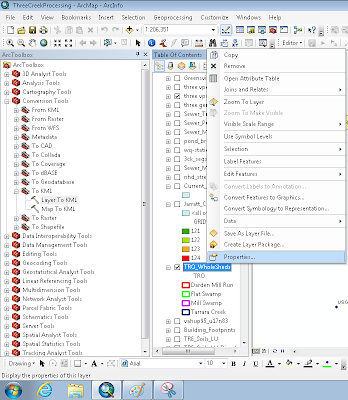
ArcMap Screenshot showing Properties and the Expanded Toolbox (next step)

3. Open ArcToolbox (Geoprocessing --> ArcToolbox) and expand the Conversion Tools heading. Expand the 'To KML' option and double click Layer To KML.

4. In the dialog that appears, under 'Layer' select the layer you want to export. Save it to a useful location you'll be able to find after saving it. Make the 'Layer Output Scale' 1.

Within Google Maps:

1. Go to maps.google.com. If you are already signed in to your Google account, great - if not, click the 'Sign In' link in the upper right corner. You MUST have a Google account of some sort in order to do this.

2. Click the My Places link in the left panel:

3. Click the red 'Create Map' button in the left panel.

4. In the fields that appear, give your map a title and description. Choose the appropriate radio button to indicate whether you want this map Public or Unlisted. Personally I like things I create to go to only my intended audience, so I usually choose Unlisted. Click the Save button if it has not already autosaved.

5. Click the Import link above the Title field.

6. In the dialog that appears, browse and find the KMZ file you exported previously from ArcMap.

7. Poof! You have a map! Click the 'Done' button at the top of the panel.

8. Now for the tricky part...there is probably an easier way to do this, but I haven't discovered it yet. To get the link to share with people, first click on the 'My Places' button at the top of the left panel. Then right-click on the map you just created and select 'Copy Shortcut' - this will copy the link to that map to your clipboard, and you can now paste it into an email or wherever else you choose.

I hope you've found this informative and as exciting as I have! Happy Mapping!

A Low Flow Conundrum - Part 2

So, building on last week's post...I'm currently dealing with a swampy area in southeastern Virginia - this is the first time I've modeled swampy/marshy areas. I took advantage of HSPF's high water table routines - new in version 12.2 of the model - to simulate these areas. Arriving at parameter values was an interesting experience, perhaps something to be discussed in a future post...a student working in the TMDL group at Virginia Tech is delving further into the sensitivity of these high water table parameters for his master's research.

One of the first oddities that struck me occurred when I generated the function tables for these watersheds. Ever since earlier research in the group demonstrated that the function table, as long as it is somewhat sound, has little effect on the overall hydrology predicted by HSPF, we have tended toward using an automated method to generate function tables based on the Natural Resources Conservation Service's hydraulic geometry curves and Digital Elevation Model (NED) information. It is preferable to gather one cross-section per modeled subwatershed, but in cases like the current one, where we have 78 subwatersheds to study, it becomes extremely costly to collect so many profiles.

So, moving forward with the NRCS data for the coastal plain region in Virginia, I noticed that the combination of bankfull depth, top width, and cross-sectional area did not yield a typical trapezoidal cross-section. Normally I use these three estimates to come up with a bottom width for the channel by assuming a trapezoidal channel geometry, but the calculations in this case yield a bottom width slightly larger than the top width. This didn't initially raise any flags for me, I made a mental note of the oddity and simply set the bottom width equal to the top width and moved on.

Unfortunately the studied streams did not have hydrology gauges, so I was unable to compare modeled hydrology with anything observed. We used a 'surrogate watershed' (that already had a TMDL completed) for which the function tables were calculated by another consulting firm (the methodology they used is not evident from the files they provided). During water quality calibration, I noticed that the streams went dry - a lot. This made no logical sense as we know the area we're studying is swampy. Further investigation showed that the free water surface evaporation from the reaches, nothing I had ever given much thought to before, was exceedingly high for the model of these watersheds. I traced the reason back to the difficulty in calculating bottom width - normally the bottom width is considerably smaller than the top width, so that while the flow is in the range of dry stream to bankfull (where it commonly stays), the surface area of the stream decreases as the water level falls, and evaporation decreases accordingly. Because I had set the bottom width equal to the top width for these swampy areas, evaporation continued at a high rate down to the last drop of water, causing the streams to go dry much faster than they should.

To solve this problem, I investigated the function tables from the surrogate watershed and adjusted ours to match their overall pattern. This involved a decrease in the surface area at near-zero flows - which makes logical sense, as when the flow is very small the water will start to move in small streams rather than spreading out across the full flat streambed. This solved the problem for 3 of the 4 study areas. In the fourth, however, it actually caused more problems. This goes back to what I mentioned previously about dealing with low flow issues - that is, setting a cutoff. When evaporation was high, the stream spent a considerable fraction of its time beneath the cutoff stages used for livestock and wildlife. That is, their contributions were removed from the stream a considerable amount of the time. When evaporation was set at a more reasonable level, the stream spent much more time above the cutoff, causing higher contributions from livestock and wildlife and thus increasing the various statistics we use to evaluate water quality calibrations.

This is a very interesting conundrum. Typically increasing flow (done in this case by decreasing evaporation) causes a decrease in bacteria concentrations (the old axiom "the solution to pollution is dilution" - outdated as we know it to be - comes to mind). This is the first time I've seen it actually INCREASE bacteria concentrations - and it is of course due to the way we use the stage cutoff to represent behavioral changes in animals.

I have used the neighboring watersheds as guides to help me set some reasonable parameters for this troublesome watershed. I am finishing up the modeling now and we'll see how well things go!

A Low Flow Conundrum - Part 1

Beginning with the Mossy Creek and Long Glade Run TMDLs, completed back in...eesh, 2004!...my colleagues and I at Virginia Tech started considering the effects of low flows on physical and behavioral changes in the stream. We noticed at that time that very low flows (Long Glade Run in particular was observed to go dry on a regular basis) cause HSPF to simulate hyper-concentrated bacteria - I typically explain this to my students as HSPF simulating flow happening down to the last little molecule of water hopping down the stream, and trying to cram millions of bacteria into that molecule. Of course in this case the concerns are with direct discharges to the stream from animals standing in the stream and illegal discharges from residences, as overland flow contributions won't be an issue at low flows (they only occur during the high flows associated with storm events) and permitted point source discharges come in with a significant volume of water that tends to prevent low flows.

The reason this happens is that HSPF simulates the stream using a function table (FTABLE) to represent the hydraulic properties of a reach. This FTABLE includes columns for depth, surface area, volume, and discharge, and HSPF enters the table for a given volume to interpolate the other three properties. As a result, the entries in the FTABLE create a series of smooth-sided stacked trapezoids. The lowest entry in the FTABLE is required to be zero volume, so HSPF will continue to interpolate flows all the way down to zero volume in the stream.

Clearly this is problematic. The first, physical, issue is that the stream bottom is not smooth - it is rough - and there is a period of time when there is still water (volume) in the reach but there is no flow, when the water is stored in a series of disconnected pools. This means from a modeling point of view that there is water, and direct discharges into that water can occur, but they will not flow downstream. Imagine a cow standing in the puddles, defecating - the cow pie will certainly contribute a large volume of bacteria to the puddle it hits, but because the puddle doesn't connect to any other puddles, the bacteria do not have the opportunity to move downstream. Additionally, the bacteria will have time to die off before the stream flow returns to a normal level. To address this physical situation, we began adding what we called a 'flow stagnation volume' to the reach - an entry in the FTABLE, immediately after the required zero flow entry, that has a small volume but no discharge. This allows the model to appropriately simulate cessation of flow when the volume falls to a level when all water is actually in a series of disconnected pools. The water and bacteria are not lost, simply held until flow increases. This will appropriately affect ALL sources of bacteria.

The second issue is a little harder to describe mathematically. This issue is a behavioral one and is twofold. First, if the water in the stream is running in a narrow rivulet, where before cows might have stood in the stream for relief from heat, insects, etc. and had their hind ends over the water, now the stream will provide little relief from heat and pests and will be a much smaller target for the defecated material to hit. This means that at some point the cows may still drink from the stream, but it is much less likely that their manure will actually be deposited in the stream. The same could be said of wildlife, though perhaps the restrictive depth would be lower because the animals are smaller. The second issue has to do with the water availability. If there is indeed an intermittent stream in a farmer's field, a logical assumption is that he must provide an alternative water source to the livestock when the stream goes dry or nearly dry. There is a lot of anecdotal evidence and some research literature to suggest that cows with alternative water sources will spend as much as 90% less time in and around the stream. Thus, if the water is low and we assume at those times the farmer must provide another water source, we can assume that the cows will be physically removed from the stream. In a similar manner, if the stream is getting low, it stands to reason that highly mobile wildlife (e.g., waterfowl, which also happen to be the worst offenders in terms of defecating in the stream) will fly away to wetter areas, again physically removing themselves from the stream.

To address this second complex behavioral issue, we institute a "stage cutoff" on animal contributions to the stream. This means in a practical sense that we export the depth of the water from the stream as an hourly timeseries, then create a multiplier from that timeseries where depths above the critical level are given a multiplier of 1 and depths below the critical level are given a value of 0. The new multiplier timeseries is then multiplied by the input direct deposit timeseries to create a filtered input timeseries for HSPF. Thus, we can represent the animals being physically removed from the stream when the flow drops.

The flow stagnation volume was first implemented in the Beaver Creek TMDL in 2005 and has been used in all subsequent TMDLs developed at or in conjunction with Biological Systems Engineering at Virginia Tech.

The stage cutoff method was first used in the Mossy Creek & Long Glade Run TMDL, and subsequently used in the Beaver Creek, Lick Creek, and Old Womans Creek TMDLs completed under my direction. It's also been used in some TMDLs developed by my peers at Virginia Tech. Unlike the flow stagnation, which is a physical representation I feel confident is applicable everywhere, I evaluate the need for the behavioral representation (i.e., the cutoff) on a case-by-case basis during water quality calibration.

I've now set the backdrop for the current conundrum I'm facing with low flows in my current project...but I think this post is long enough for now, so I'll tell you all about it next week!

Comment on Bacteria Standards... and Biosolids Update

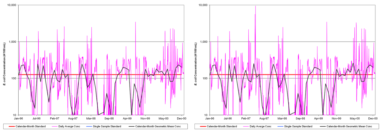
First, an update on the biosolids I wrote about last week. For my TMDL allocation scenarios, which are modeling scenarios attempting to determine the amount of pollution the water body can receive without violating standards, I set the applied load at the maximum permitted for Class B biosolids - 2,000,000 cfu/g. As I mentioned previously, I assumed a 90% loss in bacteria available for transport by surface runoff due to incorporation of biosolids within 6 hours of application. The results of this addition were not bad. In a 5-year period - with 5 biosolids application events - there were only two noticeable impacts on the bacteria concentration - can you see them in the figure below? The image on the left is without biosolids, and on the right is with biosolids. The pink line is the daily average E. coli concentration, and the black line is the calendar-month geometric mean E. coli concentration.

Overall this only added a handful of violations of the instantaneous criterion and no violations of the geometric mean criterion (red line) included in the standard for E. coli concentrations in Virginia (9VAC25-260-170). Which brings me to my second point in just a second... but first, as a general conclusion, the isolated responses shown by including biosolids were from particularly high storms in the months following application and overall did not have a large impact on modeling. Given the changes in the standard, it would appear at first glance that inclusion of biosolids at their permitted limits in the TMDL wouldn't be too difficult.

Now, the bacteria standard! 9VAC25-260-170 states that:

"The following bacteria criteria (colony forming units (CFU)/100 ml) shall apply to protect primary contact recreational uses in surface waters ...
E.coli bacteria shall not exceed a monthly geometric mean of 126 CFU/100 ml in freshwater.
...
2. Geometric means shall be calculated using all data collected during any calendar month with
a minimum of four weekly samples.
3. If there are insufficient data to calculate monthly geometric means in freshwater, no more
than 10% of the total samples in the assessment period shall exceed 235 E.coli CFU/100 ml ..."

This is more or less the same as it has always been since the switch from fecal coliform to E. coli as the indicator bacteria of choice several years ago at the urging of EPA, though at this point the Commonwealth has collected enough samples to drop the 'interim fecal coliform criteria' that were in effect until the full transition had been made. However, at long last DEQ has changed the way they require this standard to be met as part of the TMDL.

Previously, an acceptable TMDL had to have zero violations of both the geometric mean and the instantaneous (item 3 above) criteria. This is in stark contrast to the standard, which allows a 10% violation of the instantaneous criteria. As a result of this requirement, we often had to call for near-100% reductions in anthropogenic sources of bacteria - including livestock using streams for drinking water, runoff from pastures, pet waste, and failing septic systems - as well as reductions in wildlife contributions (and just how were we supposed to tell the wildlife to start using a toilet?!). This was often the only way for the model to show that there would never be a violation of the instantaneous criterion - and these reductions were often driven to extremes by a single storm event. Now, the very large issue of modeling uncertainty aside, the standard allows for a 10% violation of the criterion. My colleagues at Virginia Tech and I argued for years that we should be allowed to show a 10% violation of the criterion to match the standard.

The great news is that the Department of Environmental Quality has finally agreed with us! We can now allow a 10% violation of the instantaneous standard during modeling and still have a successful TMDL scenario. This means that we will be able to come up with much more reasonable reductions that will - hopefully - appear achievable to the watershed stakeholders. Our concern previously was that, when presented with 99-100% reductions in all bacteria sources in a watershed, the stakeholders would just give up as the goal was completely unattainable. Hopefully, seeing reductions more on the order of magnitude of 50% now, they will feel that they can really make a difference in the water quality of their local streams.

Biosolids and HSPF

Recently some of the folks I work with at Virginia Tech were contacted by the Virginia Department of Environmental Quality about modeling for biosolids. I was invited to participate in the discussion.

Biosolids pose an interesting modeling and stakeholder relations problem. They can of course have all sorts of nutrients, chemicals, metals, and of course are chock full of organic matter, but when one is developing a bacteria TMDL, these issues aren't relevant. It seems that there is some disagreement in the scientific field about the actual issues in properly treated biosolids, but that aside, it can be difficult to convince stakeholders to focus solely on the bacteria concerns related to biosolids when developing the bacteria TMDL. Other issues, if they do exist, would be addressed through the normal complaint process or perhaps in a TMDL for another pollutant. And of course if the biosolids AREN'T properly treated and applied, that opens a whole other can of worms I'm not going to consider today...

From a modeling standpoint, biosolids are difficult because their bacteria concentrations can vary quite a bit, but based on the sampling records I've seen, are almost always orders of magnitude below the standard in Virginia - 2,000,000 cfu/gram. In addition, although manure used as a fertilizer may or may not be incorporated into the soil after application, regulations specify that land-applied biosolids MUST be incorporated into the soil within 6 hours of application. This means that whatever bacteria are present in the biosolids are less available to transport by surface runoff.

To top it all off, the fields I've seen in Virginia that receive biosolids do so on a rather sporadic basis - typically the same field will not receive application every year - it will receive it once every 3 years at best. In the area I'm working with, most of the fields are 'backup' fields that are only used if all other fields available to the biosolids company have been exhausted. Additionally the area of cropland that receives biosolids is typically much smaller than the cropland in a given sub-watershed - the finest scale we typically look at in modeling. The 'standard' method of land loading used in the HSPF model is to use a load per acre per day - averaging the once every three years to a small part of the cropland area application to a load/acre/day would be completely unrepresentative of the potential impact of the concentrated application that occurs.

And finally, the biosolids, on their one day of application every three years, typically produce a significantly higher bacteria load than normally experienced by the cropland to which they're applied. Because the die-off on the land surface in HSPF is specified not as a rate but as a limit on the accumulation of the pollutant on the land surface, this raises questions on how to represent the die-off of bacteria in biosolids in HSPF.

The technique I've been using for this TMDL - using HSPF - is to represent the bacteria in biosolids as dry atmospheric deposition of a second quality constituent (where the first quality constituent is the bucket I normally use for bacteria). Representing the bacteria in biosolids as atmospheric deposition addresses the issue of application timing, and representing the bacteria in biosolids as a second quality constituent allows me to uniquely apply the biosolids to a small area of cropland without having to create an additional pervious land segment operation (this could be beneficial if one is approaching the limit on operations enforced by HSPF).

Technical gobbledygook follows... This is done by setting NQUALS to 2 for the relevant cropland PLS, setting QSOFG to 2, setting PQADFG to -1, inputting a MUTSIN timeseries with application on the appropriate dates as PQADFX through the NETWORK block, creating a new, smaller area entry for the relevant cropland PLS in the SCHEMATIC block, and using a new MASS-LINK table with that smaller area entry to that routes ONLY the second QUAL to the general bacteria bucket in the receiving RCHRES (don't want to route the first QUAL or water as they would be double-counted). I assume a 90% reduction in bacteria available to transport in surface runoff before creating the PQADFX timeseries.

To address the die-off problem, and here you really should read the "Accumulate and Remove by a Constant Unit Rate and by Overland Flow" section of the HSPF Manual, it turns out that the limit on surface accumulation (SQOLIM) doesn't actually chop things off - it is used as a ratio with the daily loading (ACQOP) to set a die-off rate. Now, the problem with this of course is that you want ACQOP to be zero - you don't want a daily loading, you only want a loading on the days when biosolids are applied. But if you set the daily loading to something like 1 or even 100 cfu/acre, this is completely insignificant compared even to the wildlife loading. So that makes your denominator in the die-off ratio non-zero. Because SQOLIM is NOT actually the limit on surface accumulation but is instead used as a ratio with ACQOP to set a die-off rate, simply set SQOLIM to be a multiple of your small ACQOP - I used 9*ACQOP to match what we use to calculate die-off for all our other bacteria on the land surface, but you can read up elsewhere (Appendix C) on how you might set an appropriate value. SQOLIM will be much much smaller than the actual load the land is receiving from biosolids, but that is okay. So far this is working well.

The final task will be representing the biosolids during allocation at an appropriate level. To be uniform with our representation of typical permitted operations (e.g., NPDES direct dischargers), we should model the application at the permitted level - the 2,000,000 cfu/gram that is rarely seen in real life. I'm planning to try this out, using the permitted level, in the next week or two as I develop allocation scenario for the TMDL I'm working on. I'll let you know how it goes...

Post-Conference Thoughts

We traveled back from Kentucky on Saturday after the ASABE 2011 Annual International Meeting. I thought the meeting was great - the keynote address was quite moving, I found several of the technical sessions informative, I spent time talking to old acquaintances, and I met some interesting new people.

I heard about some exciting new work underway in the society in developing new calibration standards for hydrologic models. This is something I feel very strongly about, having witnessed many poorly calibrated models in the past, and I am excited that the individual in charge of this effort is interested in having me participate in the standards development. I hope this might lay the groundwork for future water quality calibration standards, which I previously explored in a publication with my former colleagues at Virginia Tech.

In addition, one person I spoke with mentioned that ASABE hires individuals to help with technical editing for non-native English speakers in the journals it publishes. Having a perhaps unhealthy love of editing, I think I will follow up with the publications division at ASABE and see if I can get involved!

After the conference, we spent a couple days touring around Louisville. We visited the Kentucky Derby Museum at Churchill Downs and the Louisville Slugger Factory & Museum and took a lunch cruise on the Ohio River. All of these were quite enjoyable, I recommend them if you're in the area!

2011 ASABE International Meeting

I'm heading up today to the 2011 ASABE International Meeting in Louisville, Kentucky. I haven't been to Kentucky before, so I'm excited about the trip. I'm also looking forward to catching up with old friends, making some new acquaintances, and learning more about current events in the industry. I'm also very excited to share the news about my new business, Zeckoski Engineering, with my peers.

I've been thinking about Zeckoski Engineering for quite a while and have finally decided to take the plunge and try out working for myself. I've been working remotely for two clients - Virginia Tech and Timmons Group - ever since I finished working with CTEH on the BP Deepwater Horizon oil spill response. The setup with both of these clients has been in a more traditional employer-employee relationship, but I was able to work from home, set my own schedule, and largely set my own goals, and I've found it to be a very rewarding experience. I think I have a lot to offer in this economic climate to companies that need modeling, GIS work, or simple software engineering tools developed but perhaps don't want the long term commitment of a permanent employee.

So if you're going to the international meeting, please stop me and say hi! I can't wait to meet you!